Tutorial

Importing packages

import warnings
warnings.filterwarnings('ignore')

import tmplot as tmp
import pickle as pkl
import pandas as pd

Importing data

Let’s take the BTM model trained on a test dataset (SearchSnippets) as an example. We will begin with reading it from a file:

with open('data/model_btm.pkl', 'rb') as file:
    model = pkl.load(file)

docs = pd.read_csv('data/SearchSnippets.txt.gz', header=None).values.ravel()

Matrices

Researchers working with topic models often need to obtain phi (words vs topics probability) and theta (topics vs documents probability) matrices. Tmplot provides two functions for getting these matrices from tomotopy, bitermplus, and gensim models.

Phi matrix

Note that you will need to pass a vocabulary for a gensim model.

phi = tmp.get_phi(model)
phi.head()

topics	0	1	2	3	4	5	6	7
words
aaa	3.195102e-08	3.012856e-08	3.047842e-08	3.542745e-08	3.836165e-08	2.961217e-08	2.362519e-08	4.831267e-08
aaas	3.837318e-05	3.012856e-08	3.047842e-08	3.542745e-08	3.836165e-08	5.922729e-04	6.144912e-05	2.903592e-05
aaron	3.195102e-08	3.012856e-08	3.047842e-08	3.542745e-08	4.296888e-04	2.961217e-08	2.362519e-08	4.831267e-08
aau	3.195102e-08	3.012856e-08	3.047842e-08	3.542745e-08	3.836165e-08	2.961217e-08	2.362519e-08	4.203686e-04
abbreviations	7.990951e-05	3.163800e-04	3.047842e-08	3.542745e-08	3.836165e-08	2.961217e-08	2.386144e-06	4.831267e-08

Theta matrix

tmp.get_theta(model).head()

docs	0	1	2	3	4	5	6	7	8	9	...	990	991	992	993	994	995	996	997	998	999
topics
0	0.354702	0.294777	0.178074	0.332888	0.596412	0.726975	0.099094	0.257602	0.532725	0.471059	...	0.007651	0.085897	0.025840	0.019194	0.033898	0.020408	0.030728	0.036133	0.084323	0.024301
1	0.000245	0.007173	0.021324	0.019411	0.029472	0.008740	0.011804	0.036323	0.011349	0.003909	...	0.069988	0.263869	0.058431	0.227196	0.022920	0.021660	0.040932	0.060534	0.150018	0.071271
2	0.003073	0.057144	0.013837	0.014514	0.011813	0.002588	0.000247	0.027391	0.002325	0.005435	...	0.007558	0.014669	0.014206	0.002697	0.008854	0.017299	0.014710	0.027672	0.061375	0.011318
3	0.003678	0.029281	0.010010	0.001287	0.027349	0.004351	0.018189	0.085879	0.011453	0.002965	...	0.007010	0.022462	0.007516	0.006018	0.001193	0.007400	0.007335	0.021119	0.012309	0.006168
4	0.000927	0.035162	0.001736	0.319421	0.024606	0.042996	0.019524	0.036119	0.001910	0.039332	...	0.016587	0.056386	0.005925	0.003503	0.001620	0.006468	0.004151	0.018374	0.008712	0.087364

5 rows × 1000 columns

Documents

Here is how you can get documents with maximum probabilities \(P(t|d)\) for each topic:

tmp.get_top_docs(docs, model=model)

	topic0	topic1	topic2	topic3	topic4	topic5	topic6	topic7
0	speakeasy speedtest speakeasy speed test test ...	links jstor sici sici jstor postwar consumptio...	imdb name julia roberts julia roberts imdb mov...	guitars bodies amps guitars strings	vcic unc edu vcic venture capital investment c...	washington edu drivers device drivers device d...	apache api dom document document xml standard ...	hypotheses hypotheses author illustrates hypot...
1	speedtest bandwidth speed test bandwidth speed...	econpapers repec article econpapers postwar co...	celebrities cruise celebrity tom cruise tom cr...	louis french fashion designer designer manufac...	national venture capital association foster un...	manufactures parallel serial drives	schools dom default xml dom tutorial xml docum...	surreal surreal
2	home bandwidth broadband speedtest bandwidth c...	findarticles articles consumption consumer exp...	imdb name tom cruise tom cruise imdb movies ce...	fashion designers default fashion designers fa...	san jose mercury news venture capital expanded...	leonardo leonardo vinci inventor information c...	access cards ieee access	allposters surrealism posters surrealism poste...
3	home bandwidth broadband speedtest bandwidth c...	financial financial international health insur...	absolutely roberts absolutely julia roberts ph...	fashion designers audio fashion designer net f...	seattlepi nwsource venture seattle venture cap...	journals searching biomedical journals engine ...	generator xml generator sample xml instance do...	hypotheses hypotheses nature research hypothes...
4	portfolio shareholder services manage investme...	consumption consumer rights consumption consum...	imdb title imdb movies celebs	fashion fashion designers fashion designers fa...	venture capital journal listening model ventur...	lwn articles driver lwn device drivers kernel ...	reference standard template library standard t...	allposters beatles posters beatles prints allp...

Visualization

tmplot takes much from LDAvis, but also extends the functionality with a number of algorithms and metrics for plotting topics and terms. tmplot is based on ipywidgets and Altair (Vega-backed package for nice plots).

Topics

First, we need to calculate the coordinates of topics based on intertopic distance values. By default, the combination of t-distributed Stochastic Neighbor Embedding and symmetric Kullback-Leibler divergence is used to calculate topics coordinates in 2D, but a number of other metrics and algorithms are also available (see tmplot.get_topics_dist and tmplot.get_topics_scatter functions for additional information).

topics_coords = tmp.prepare_coords(model)
topics_coords.head()

	x	y	topic	size	label
0	-41.183987	-30.480648	0	21.160233	0
1	-11.704910	-34.631725	1	4.265470	1
2	-56.292171	-4.832846	2	20.599346	2
3	9.921317	-14.181945	3	7.176289	3
4	-45.702721	22.987968	4	4.535249	4

Plotting topics:

tmp.plot_scatter_topics(topics_coords, size_col='size', label_col='label')

Words (or terms)

tmplot also uses terms relevance that was introduced by Sievert and Shirley (2014) for sorting terms.

terms_probs = tmp.calc_terms_probs_ratio(phi, topic=0, lambda_=1)

tmp.plot_terms(terms_probs)

Documents

top_docs_topic0 = tmp.get_top_docs(docs, model=model, docs_num=2, topics=[0])
top_docs_topic0

	topic0
0	speakeasy speedtest speakeasy speed test test ...
1	speedtest bandwidth speed test bandwidth speed...

The following output is used within the interactive interface that we will explore shortly:

tmp.plot_docs(top_docs_topic0)

	topic0
0	speakeasy speedtest speakeasy speed test test speed internet connection speakeasy speed test
1	speedtest bandwidth speed test bandwidth speed test bandwidth bandwidth speed internet service

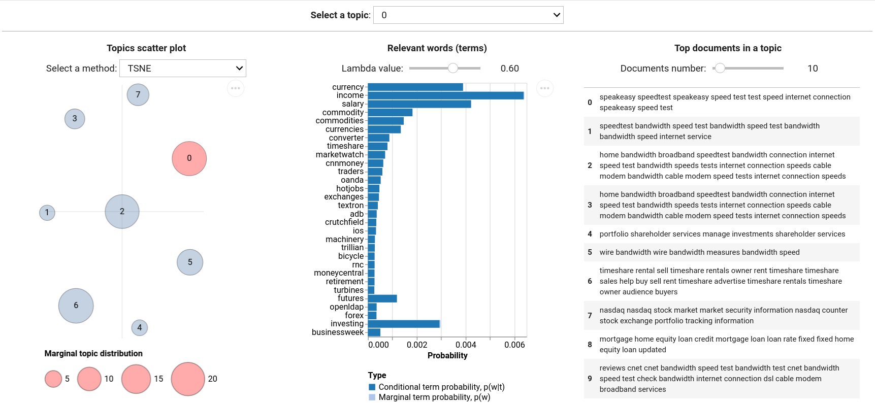
Interactive report interface

To run the report interface, just call tmplot.report() function with your model and docs. You can tweak most of the hidden parameters using keyword arguments (see function docstring).

tmp.report(model, docs=docs, height=400, width=250)